Applications can generate data in formats that aren’t quite useful – glomming multiple fields together to make something unusable. And asking people to type information can yield inconsistent results – is my name Lisa Rushworth, Lisa J Rushworth, or just Lisa? Excel has several functions that allow you to produce consistent, usable data (without copy/pasting or deleting things!)
Flash Fill
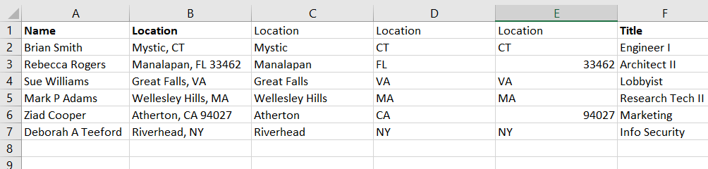
Flash Fill will try to figure it out for you. Add an empty column (or more) and manually type one or two values. On the “Data” ribbon bar, select “Flash Fill” and Excel will use the data you’ve entered into the row to figure out what should go in the rest of the row.
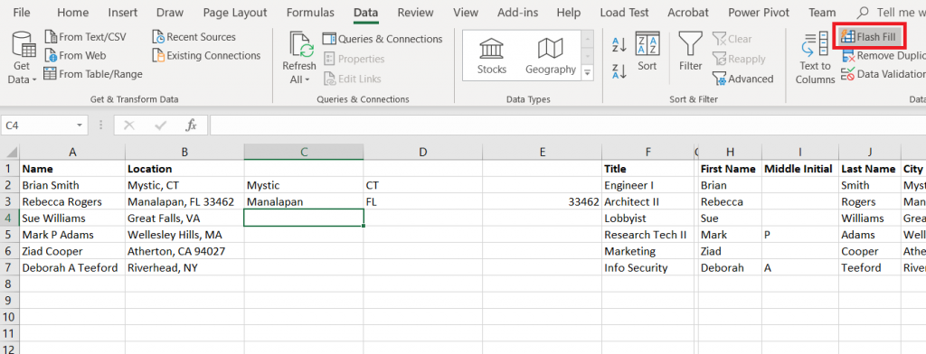
The guesses aren’t 100% accurate – especially if your information is not consistent – but it’s a lot easier to delete the handful of things that are obviously not zip codes …
Than to work out a formula that extracts the same information
Text to columns
Text to columns uses the fixed-length file and delimited file import wizard on a column of data – essentially treating that column as a file to be imported. In this example, a DateTime value is provided in a way that Excel only sees it as a string. And, frankly, I am not interested on the exact hundredth of a second the event occurred. What I really want to do is group these creation dates by day, so all I need is the date component.
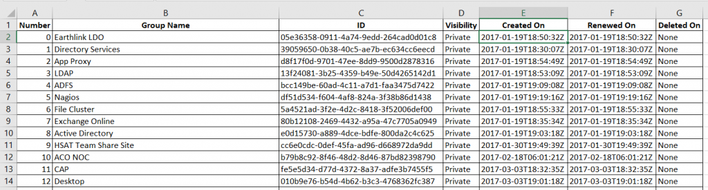
If you want to retain all the data, you’ll need to insert empty columns to the right – otherwise the data being split out can overwrite existing data. In my case, I only want to keep one of the new columns.
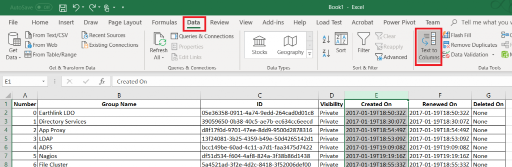
Highlight the column that holds your data. On the “Data” ribbon, select “Text to columns”
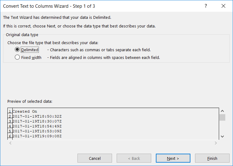
Select if the column should be split based on a fixed width definition or a delimiter and click ‘Next’
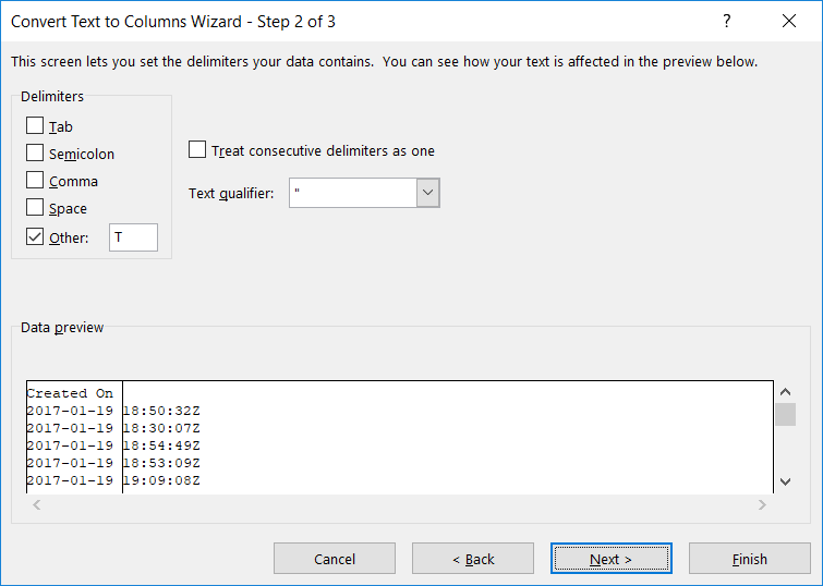
Indicate the proper delimiter – in this case, I need to use ‘Other’ and enter the letter T. A preview of the split data will appear below – make sure it looks reasonable. Click “Next”.
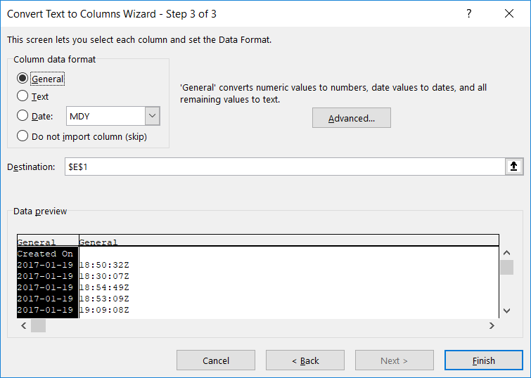
For each new row, you can specify a data type. Or leave the type set to “General” and Excel will try to figure it out.
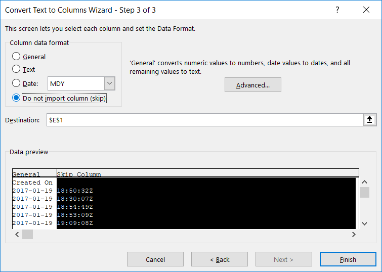
If you do not need to retain the data, select “Do not import this column (skip)”. Click “Finish” to split your column.
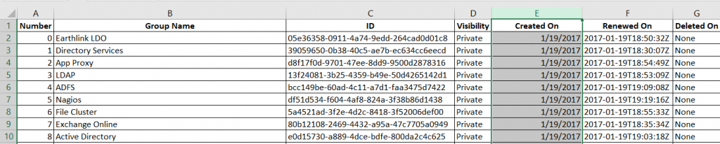
Voilà – I’ve got a usable date value.
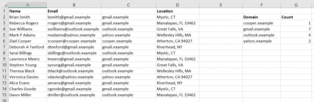
Notice, though, I have lost my original data. If you want to retain the original data, create a copy of the column. In this example, I want to know how many e-mail addresses use each domain, but I want to have the e-mail addresses in a recognizable and usable format too.
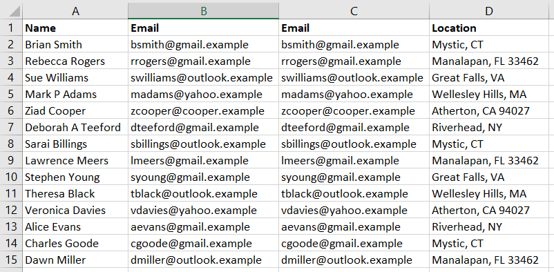
Text to columns will still replace the values from the selected column. But the copy will contain the original text.
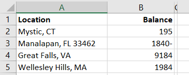
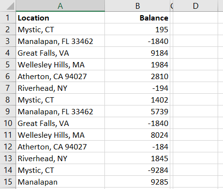
You can even use Text to columns to sort out odd data that doesn’t actually get split into multiple columns. In this example, negative values have the minus sign after the number … which isn’t actually a negative number and isn’t usable in calculations.
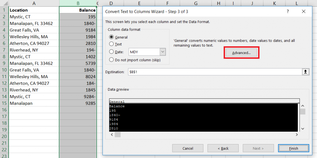
Pick a delimiter that doesn’t appear in your data, and you’ll only have one column. When selecting the data format, click “Advanced”
Make sure the “Trailing minus for negative numbers” checkbox is checked and click OK.
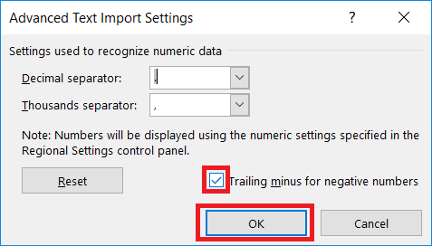
And we’ve got negative numbers
Right, Left, Mid, and Search Functions:
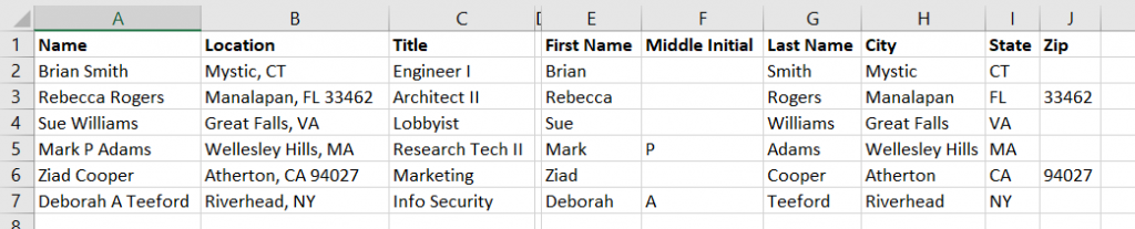
You can also use the Search function in conjunction with Right, Left, and Mid to extract components of column data. In this example, we have first and last names. Since there are a few middle initials in there, we cannot just split on the space character.

These formulae aren’t perfect – Mary Ann will have ‘Mary’ as a first name – but
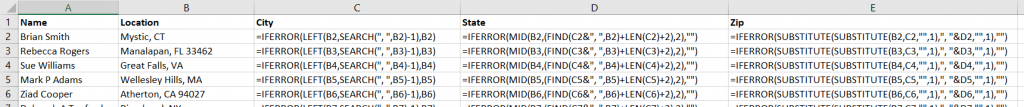
Working out where to start the text extraction and the number of characters to extract can get complex. I’ll usually include the Substitute function to simplify things a little – the zip code, in this case, is whatever is left over after we find the city and state.
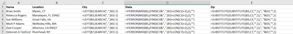
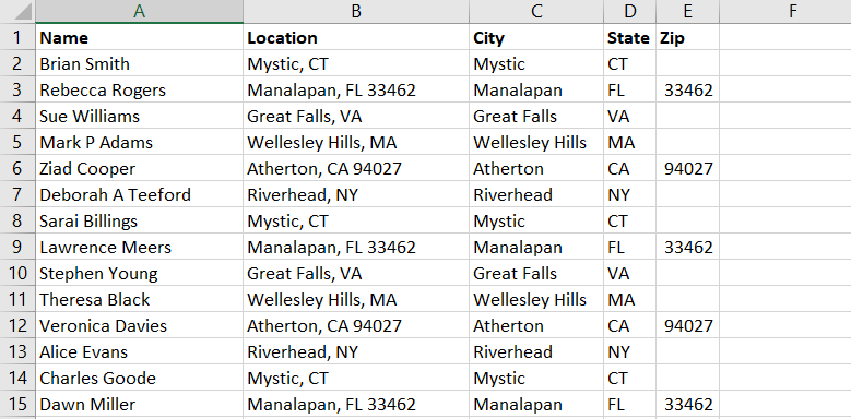
Producing columns with the city, state, and zip code from the ‘Location’ column.