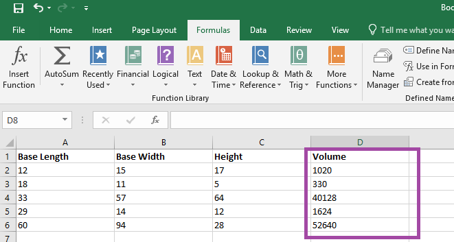
Formulae in Excel aren’t always easy to decode – even a relatively simple formula, like the volume of a right rectangular pyramid below, can be a little cryptic with the A2 type cell identifiers.
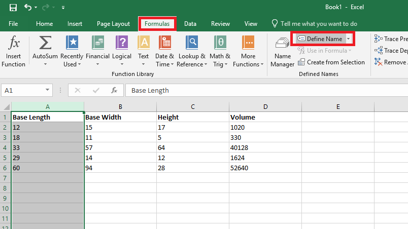
You can name ranges and use range names to make a formula easier to understand. Highlight a data set – in this case, I am highlighting the “length” values – column A. On the “Formulas” ribbon bar, click on “Define Name” (you don’t need to hit the inverted caret on the right of the button – just click the ‘define name’ text).
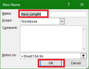
Supply a name for the range – in this case, I am calling it “Base_Length” (range names need to start with a letter or underscore and cannot contain spaces). Click OK to save the range name. Repeat this operation with all of the other data groups – in my case, I named Column B “Base_Width” and Column C “Height”.
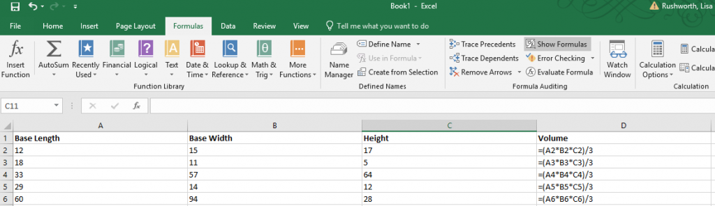
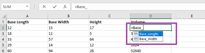
Use the name instead of the cell identifier – as you type your formula, the range names matching your typed text will appear.
It is now a lot clearer what this formula means – base length times base width time height all divided by three. Which is the formula to calculate the volume of a right rectangular pyramid.
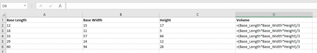
The calculated answer is the same either way – but this makes it easier to figure out what exactly you were computing when you open the spreadsheet again in six months 😊 (Or share the spreadsheet with others).